
Publicerat av Sensorbee den · 5 min läsning
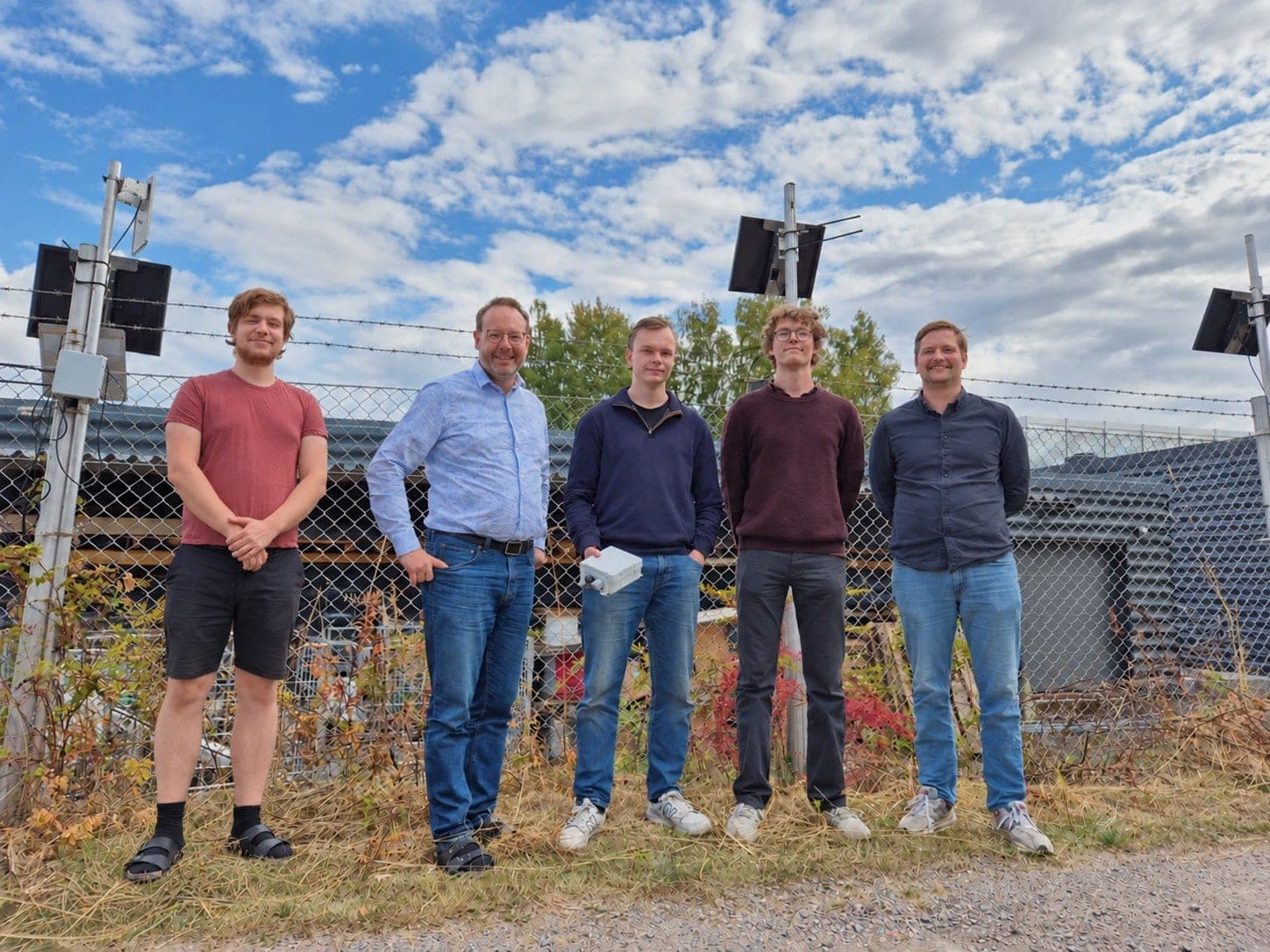
Summer interns Love Hedbom and Albin Söderteg with the Sensorbee team, summer 2026. Behind them, solar-powered Sensorbee units on the fence of the test site.
Every summer since 2024, Sensorbee has taken on engineering students to work on one question: how do we get more accurate gas readings out of low-cost electrochemical sensors? This year's interns, Love Hedbom and Albin Söderteg, picked up where the 2025 team left off. They were given a year of new field data, the calibration code that runs in production today, and a brief to improve it.
By August they had presented a machine-learning calibration model that outperforms our current method on both nitrogen dioxide (NO2) and nitric oxide (NO), packaged as a small library our backend team can run. This article summarises what they did, what did not work, and what happens next.
The brief
The Air Pro 2 measures gases with plug-in electrochemical modules such as our NO2 sensor. These sensors are compact and affordable, but their raw signal drifts with temperature, humidity and age. In production, Sensorbee corrects for this with an automatic baseline calibration built on a Kalman filter. It needs no reference instrument, which is what makes it usable on a construction site or a lamppost.
The internship had four objectives:
- ·Optimise the existing calibration. Re-tune the baseline correction against the latest data so it stays robust across seasons.
- ·Investigate sensor ageing and drift. Find out how sensitivity changes over a sensor's life and whether it can be compensated.
- ·Explore machine learning and sensor fusion. Test whether a model that learns from temperature, humidity and co-located gas channels can beat conventional signal processing.
- ·Refine signal integrity. Separate real concentration changes from noise and spurious data points.
The dataset came from Sensorbee units co-located with reference-grade analysers at three sites, two in Stockholm and one in Linköping, with the Stockholm reference data supplied by SLB Analys, the City of Stockholm's air quality unit. It covered around 17 months at five-minute resolution, roughly 925 station-days in total.
Most of the time went into the data
The first surprise was how much effort clean data takes. Before any modelling, Love and Albin had to align sensor and reference series that were recorded at different intervals, reconcile time zones and daylight-saving changes, and manually handle gaps and step changes in the sensor record. They describe it as the least glamorous and most important part of the project. A model trained on misaligned data learns the misalignment.
Three approaches that did not work
Part of the value of a research internship is ruling things out with evidence. Three ideas were tested and set aside:
- ·Frequency-domain transfer function. The idea was to describe the relationship between sensor and reference signals in the frequency domain and translate one into the other. The resulting transfer function looked like white noise, with no usable structure.
- ·Outlier rejection. Removing physically implausible jumps in gas or temperature readings seemed sensible, but the gaps it created broke the Kalman filter's state tracking and made results worse.
- ·Low-pass filtering. Filtering out high-frequency noise improved the average error, but at the cost of slower and weaker response to short, high-concentration peaks. For air quality work, the peaks are often exactly what matters.
Sensor drift is seasonal, and tied to temperature
On ageing, the data pointed to sensor gain falling over time, but the pattern tracked the seasons more than the calendar. Gain showed a strong inverse relationship with temperature, explaining roughly two-thirds of the variation. With 17 months of data the team could not separate a true ageing trend from a repeating seasonal cycle, and they say so plainly. That question is now on the list for a future project, and Sensorbee has extended reference-data retention to three years to make it answerable.
Tuning the existing calibration
Sweeping the parameter space of the current Kalman baseline correction produced a modest improvement, reducing mean squared error on NO2 from around 16 to 14.3. The team also proposed seasonal parameter sets and a shorter lookback window as follow-ups. Useful, but not a step change.
The step change: a gradient-boosted model
The result that changed the conversation was a gradient-boosted tree model. Rather than modelling the sensor's physics explicitly, it learns the non-linear relationship between raw sensor output and the reference value from data. It uses 24 features, all derived from a small set of inputs already available on every unit: the raw NO and NO2 channels, temperature, humidity, time of day and year, and modelled solar intensity at the unit's location, which stands in for ozone where no ozone reference is available.
The model was validated two ways. Cross-validation (CV) tests it on unseen time periods at sites it has trained on. Leave-one-site-out (LOSO) is the harder test: the model is trained on two sites and evaluated on a third it has never seen, which is closer to how it would be used in the field.
NO2 (root mean squared error, ppb)
| Method | RMSE | R² |
|---|---|---|
| Raw sensor | 4.97 | −0.05 |
| Current Kalman baseline | 3.78 | 0.39 |
| Gradient-boosted model, CV | 2.35 | 0.76 |
| Gradient-boosted model, LOSO | 3.02 | 0.61 |
NO (root mean squared error, ppb)
| Method | RMSE | R² |
|---|---|---|
| Raw sensor | 42.6 | −35.0 |
| Current Kalman baseline | 23.1 | −9.6 |
| Gradient-boosted model, CV | 5.04 | 0.50 |
| Gradient-boosted model, LOSO | 6.33 | 0.21 |
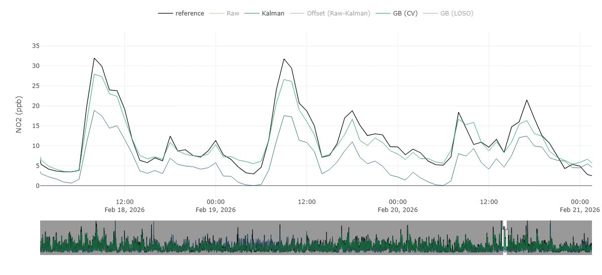
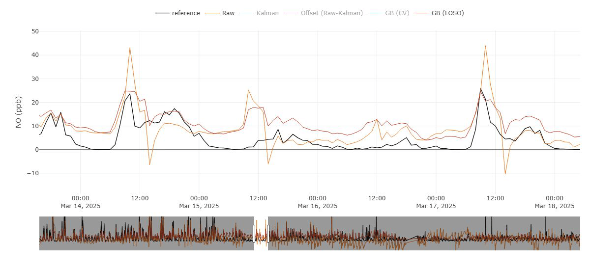
On NO2 the model cuts error by around a third against the current method even at a site it has never seen. On NO the gain is larger still, because the electrochemical NO signal is far harder to correct with baseline tracking alone. The model was also noticeably better at following short, high-concentration peaks, the case where filtering approaches struggled.
What happens next
The interns delivered the model as a small Python library with two parts: a stateless runtime the backend calls per reading, and a one-command retraining script for when new reference data arrives. Both share the same feature code, so what is trained is what is served. It needs no special infrastructure.
That library has been handed to our backend team for evaluation and integration into Sensorbee Cloud. In parallel, the proposed improvements to the existing Kalman correction are planned, along with a reporting mechanism so we can track calibration performance continuously rather than at review points.
Further work the team recommended:
- ·Extend the approach to other gases, starting with carbon monoxide.
- ·Feed in measured ozone where a reference is available, instead of the solar proxy.
- ·Explore fusing two NO2 sensors on one unit.
- ·Build lightweight versions that could run on the device itself.
Thank you, Love and Albin
Research internships are a real part of how Sensorbee develops its products. The 2026 project produced a deployable result, an honest account of three dead ends, and a clear set of open questions for the 2027 team. Our thanks to Love Hedbom and Albin Söderteg for a focused summer's work, and to SLB Analys for the reference data that made the work possible.
Interested in how Sensorbee approaches sensor accuracy? Get in touch or download the catalogue.

Sensorbee
Environmental Monitoring