Smog Monitoring with Air Quality Sensors

Seven million people die prematurely each year from air pollution, according to the World Health Organisation. A significant proportion of those deaths occur in cities where smog, a mixture of ground-level ozone, nitrogen dioxide, sulphur dioxide, and fine particulate matter, reaches concentrations that damage human health within hours of exposure.

Smog is not a problem confined to developing nations. European cities regularly experience smog events during summer heat waves and winter temperature inversions. London, Paris, Milan, and Warsaw have all declared air quality emergencies in the past five years. In the UK, DEFRA issues air pollution alerts when ozone and PM2.5 levels exceed moderate thresholds, affecting millions of residents.

What Smog Is and Why It Forms

Smog forms when pollutant gases and particles interact with sunlight and atmospheric conditions. There are two distinct types relevant to urban monitoring.

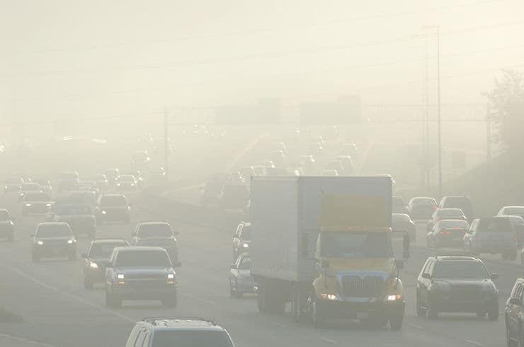
Photochemical smog occurs when nitrogen oxides (NOx) and volatile organic compounds (VOCs) react in sunlight to produce ground-level ozone (O3). This is the brown haze visible over cities on hot, still days. The WHO's 2021 updated Air Quality Guidelines set the ozone peak season mean at 60 µg/m³ (reduced from the previous 100 µg/m³), with an 8-hour mean guideline of 100 µg/m³. Concentrations above these levels irritate airways and trigger asthma attacks.

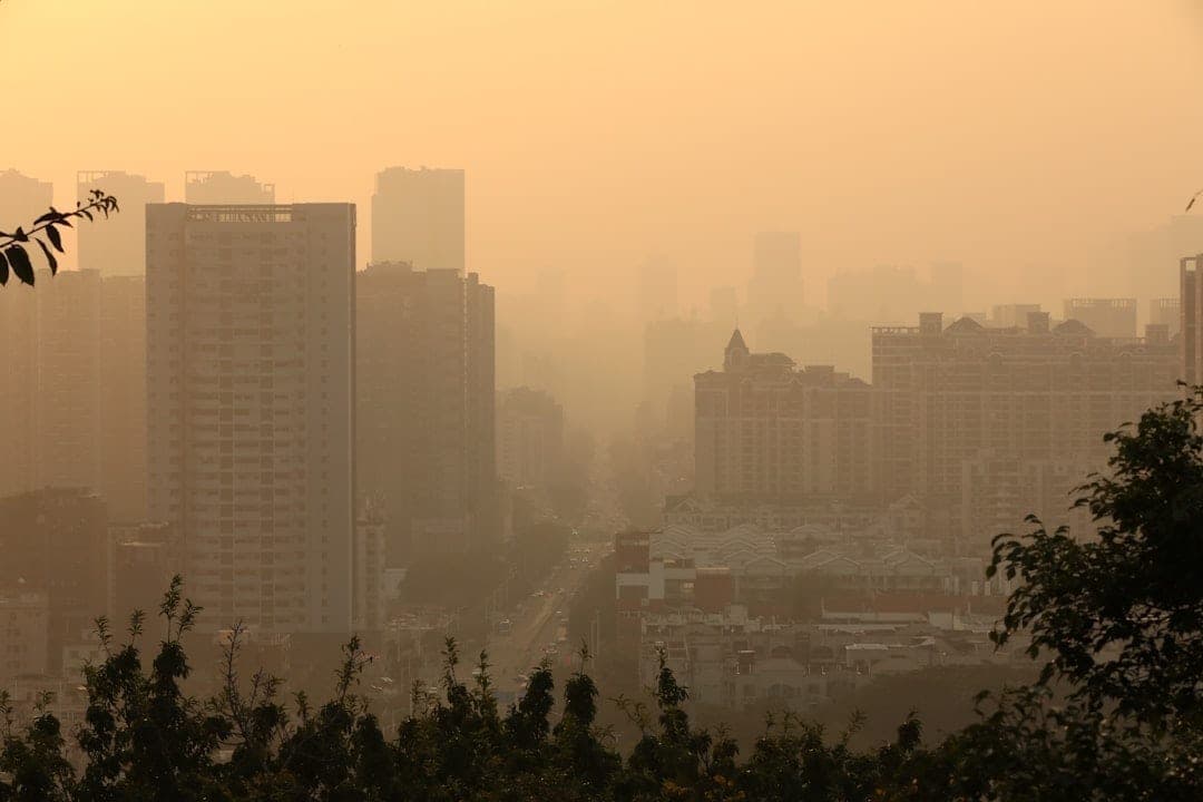
Winter smog forms during temperature inversions, where cold air at ground level is trapped beneath a warmer layer, preventing pollutant dispersal. PM2.5 from vehicle exhausts, domestic heating, and industrial emissions accumulates to dangerous levels. During London's 2017 winter smog episode, PM2.5 concentrations exceeded 60 ug/m3 in parts of the city, six times the WHO annual guideline.

Both types share a critical characteristic: they are highly localised. A street canyon in a city centre may experience PM2.5 levels three to five times higher than a park 500 metres away. This spatial variation is precisely what makes smog difficult to monitor with conventional approaches.

The Limitations of Conventional Monitoring

Most cities rely on a small number of reference monitoring stations to assess air quality. These stations provide accurate measurements, but their design creates fundamental blind spots when monitoring smog.

Sparse spatial coverage. A typical UK city operates five to 15 reference stations across its jurisdiction. Smog concentrations vary dramatically over distances as short as 100 metres due to traffic patterns, building geometry, and wind effects. Stations spaced kilometres apart miss these variations entirely.

Fixed positions. Reference stations are permanent installations requiring mains power, climate-controlled enclosures, and regular technician access. They cannot be repositioned to investigate emerging smog sources or placed at locations where infrastructure does not exist.

Delayed data. Many reference networks report hourly or daily averages. A 30-minute ozone spike from a photochemical event or a PM2.5 surge from a construction site may not appear in the data with sufficient resolution to trigger an intervention.

High cost per point. At EUR 120,000 to EUR 300,000 per station, expanding reference networks to achieve meaningful spatial coverage is financially impractical for most local authorities.

These constraints leave cities managing smog with incomplete data. Interventions such as traffic restrictions or industrial controls are applied broadly rather than targeted at the streets and hours where smog actually exceeds thresholds.

How Dense Sensor Networks Change Smog Monitoring

The alternative to sparse, expensive reference networks is dense deployment of lower-cost, independently certified sensors. A network of 40 to 100 sensors across a city achieves spatial resolution that reference stations cannot match, at a fraction of the cost.

Dense networks enable three capabilities essential for effective smog management.

Source identification. When sensors are spaced 200 to 500 metres apart, pollution gradients become visible. A consistent PM2.5 elevation downwind of a specific junction, factory, or port identifies the source for targeted action. Without spatial data, all sources are treated equally.

Event detection. Real-time data from distributed sensors captures short-duration pollution spikes that hourly averages mask. A 20-minute ozone exceedance during a photochemical event triggers an immediate alert rather than appearing as a minor blip in the daily average.

Intervention evaluation. When a city implements a traffic restriction or an industrial facility adjusts operations, dense monitoring networks measure the downstream effect within hours. Reference stations, often located away from the intervention zone, may not register a measurable change.

Multi-Pollutant Measurement for Smog Analysis

Smog is not a single pollutant. Effective monitoring requires simultaneous measurement of the gases and particles that combine to form it.

Particulate matter (PM1, PM2.5, PM10). The solid and liquid particles that constitute visible smog and cause the most direct health damage. PM2.5 penetrates deep into lung tissue and enters the bloodstream. The Sensorbee particle matter module measures all three fractions simultaneously.

Nitrogen dioxide (NO2). A primary combustion pollutant from vehicles and industrial processes that both damages health directly and serves as a precursor to ozone formation. NO2 sensors track this critical parameter in real time.

Ground-level ozone (O3). Formed through photochemical reactions, ozone is the defining component of summer smog. Monitoring O3 alongside its precursors (NOx and VOCs) reveals whether conditions favour smog formation before it becomes visible.

Sulphur dioxide (SO2). A marker of industrial and shipping emissions, SO2 contributes to winter smog and forms secondary particulates through atmospheric chemistry.

Volatile organic compounds (VOCs). Industrial solvents, fuel vapours, and natural sources emit VOCs that react with NOx in sunlight to produce ozone. Measuring VOC levels identifies missing pieces of the smog formation puzzle.

Carbon monoxide (CO). A combustion indicator that helps distinguish traffic-related pollution from other sources. CO monitoring supports source attribution in complex urban environments.

The Sensorbee Air Pro 2 measures all of these parameters from a single unit, eliminating the need for separate instruments for each pollutant. This integrated approach provides the complete dataset needed to understand smog formation, persistence, and dispersal.

Deployment Scenarios for Smog Monitoring

Different urban and industrial environments require different monitoring approaches. Sensor networks can be configured for each scenario.

Urban street-level networks

Cities deploying sensors at 200 to 500 metre intervals along major roads, junctions, and pedestrian zones create a real-time pollution map. Data feeds into cloud dashboards where officials track which streets exceed thresholds and at what times. This enables targeted interventions: restricting heavy vehicles on a specific corridor during morning hours, for example, rather than applying blanket restrictions across the city.

Industrial perimeter monitoring

Factories, refineries, and waste processing facilities deploy sensors along their site boundaries to monitor fence-line concentrations. Real-time SO2, NO2, and PM2.5 data demonstrates whether emissions contribute to local smog episodes or remain within permit conditions. A wind sensor at each monitoring point provides directional context for source attribution.

Construction site dust management

Large construction projects generate fugitive dust that contributes to localised PM10 and PM2.5 elevation. Continuous perimeter monitoring with automated alerts enables site managers to implement mitigation measures, such as water suppression, road sweeping, or activity suspension, before dust reaches neighbouring properties.

Transport corridor assessment

Airports, ports, and major road corridors concentrate emissions from thousands of vehicle movements daily. Monitoring networks along these corridors quantify the pollution contribution and track whether mitigation measures, such as shore power at ports or low-emission zones around airports, achieve measurable reductions.

Solar Power and Cellular Connectivity

Two practical constraints have historically limited where air quality sensors can be deployed: access to mains electricity and wired data connections. Both constraints are eliminated by solar-powered sensors with cellular connectivity.

The Air Pro 2 operates entirely on solar power with battery backup, maintaining continuous measurement through extended cloudy periods. This means sensors can be placed at the actual locations where smog concentrations are highest, not where electrical infrastructure happens to exist.

Cellular data transmission via NB-IoT or LTE-M provides reliable connectivity without wired networks. Data streams to a cloud platform in real time, where it is stored, visualised, and available for alert generation. Built-in data buffering ensures no measurements are lost during temporary connectivity gaps.

This combination of solar power and cellular connectivity transforms deployment logistics. A sensor can be installed on a lamp post, building facade, fence post, or temporary structure in under 10 minutes with no site preparation, no electrical contractor, and no data cable installation.

From Data to Action

Monitoring data only reduces smog exposure when it drives specific decisions. Effective smog monitoring systems connect measurement to action through several mechanisms.

Threshold alerts. When PM2.5 exceeds 25 ug/m3 or ozone exceeds 100 ug/m3 at any sensor location, automated notifications reach responsible personnel. Alerts can trigger predefined response protocols, from construction site dust suppression to traffic management centre actions.

Trend analysis. Weekly and seasonal patterns reveal when and where smog concentrations are increasing. A city observing rising NO2 at a specific junction during school run hours can target that location with traffic calming or school travel plan improvements.

Compliance reporting. Regulatory bodies require documented evidence of air quality conditions and the effectiveness of management measures. MCERTS-certified monitoring data provides the evidence standard authorities expect.

Public communication. Real-time air quality data published to residents builds awareness and enables individual protective actions. People with respiratory conditions can avoid high-pollution areas during smog events when spatial data identifies which streets are affected.

Frequently Asked Questions

What causes smog in UK cities?

UK smog results from two main processes. Summer smog forms when vehicle NOx emissions and VOCs react in sunlight to produce ground-level ozone. Winter smog occurs during temperature inversions that trap PM2.5 from vehicles, heating systems, and industry near ground level. Both types are worsened by street canyon effects that limit pollutant dispersal in dense urban areas.

How many sensors are needed to monitor smog effectively?

Coverage requirements depend on city size and pollution source density. For a mid-sized UK city (population 200,000 to 500,000), a network of 30 to 60 sensors at 200 to 500 metre intervals along major roads and around key sources provides sufficient spatial resolution to identify hotspots and evaluate interventions. This can be expanded as monitoring priorities evolve.

Can air quality sensors replace reference monitoring stations?

No. Dense sensor networks complement reference stations rather than replace them. Reference stations provide the highest accuracy measurements needed for legal compliance assessment. Indicative sensor networks, particularly those with MCERTS certification, provide the spatial coverage needed to understand where pollution varies across a city and to direct targeted interventions.

What is the difference between PM2.5 and PM10?

PM2.5 refers to particulate matter with a diameter of 2.5 micrometres or less. PM10 refers to particles up to 10 micrometres in diameter. PM2.5 is more dangerous because smaller particles penetrate deeper into the lungs and can enter the bloodstream. Both are regulated under UK and EU air quality standards, with PM2.5 receiving increasingly strict limits due to its stronger association with cardiovascular and respiratory disease.